How to Draw a Sloping Surface in Plan

Slope with H2o Table

1. Introduction

The simplest 3D slope contour is one with a constant profile.

In this tutorial we will create a simple extruded slope, run the analysis, so add a water table and re-run the analysis.

2. Projection Settings

Let's first await at the Project Settings dialog. This allows you to configure the master settings for your analysis.

Select: Analysis > Project Settings

Select the [Units] tab. Make sure the Units = Metric, stress as kPa.

Select the [Methods] tab. We will utilize the default selected methods (Bishop and Janbu).

Nosotros volition be using the default settings. Select OK or Cancel.

3. Geometry

Select the Geometry Workflow tab .

For the purposes of this tutorial, we will create a second gradient contour with the Draw Polyline tool using two different methods:

1. Importing a .csv file, and
2. Inbound coordinates

Select: Geometry > Polyline Tools > Draw Polyline

Nosotros want to define the coordinates of the slope profile in the YZ vertical plane. Since the default setting is set to the XY plane, make sure to select the YZ Aeroplane Orientation selection in the sidebar on the left side of the screen.

Importing a .csv file

Select the Edit Table button in the Coordinate Input area of the sidebar.

The Edit Polyline dialog should open. You can import csv files past selecting .

Yous should see the file 'polyline_coordinates.txt' in the tutorial folder. Later on you've opened the .txt file the Import CSV File dialog appears. Make sure to select Tab in the Data Delimiter dropdown.

Y'all should now see a table of values. Select OK to become back to the Edit Polyline dialog.

At present nosotros will delete the polyline coordinates and testify how to enter the coordinates manually instead.

To delete the coordinates just highlight the tabular array and select the Delete Rows icon .

Entering Coordinates

In the Edit Polyline dialog, select the Append Rows button and add 7 rows, then click OK. Enter the following coordinates in the dialog and select OK:

U	Five
0	0
130	0
130	50
80	l
50	30
0	30
0	0

Select the greenish check marker at the top of the Depict Polyline dialog.

Alternatively, if you were working with the viewports you tin r ight-click the mouse and select Washed.

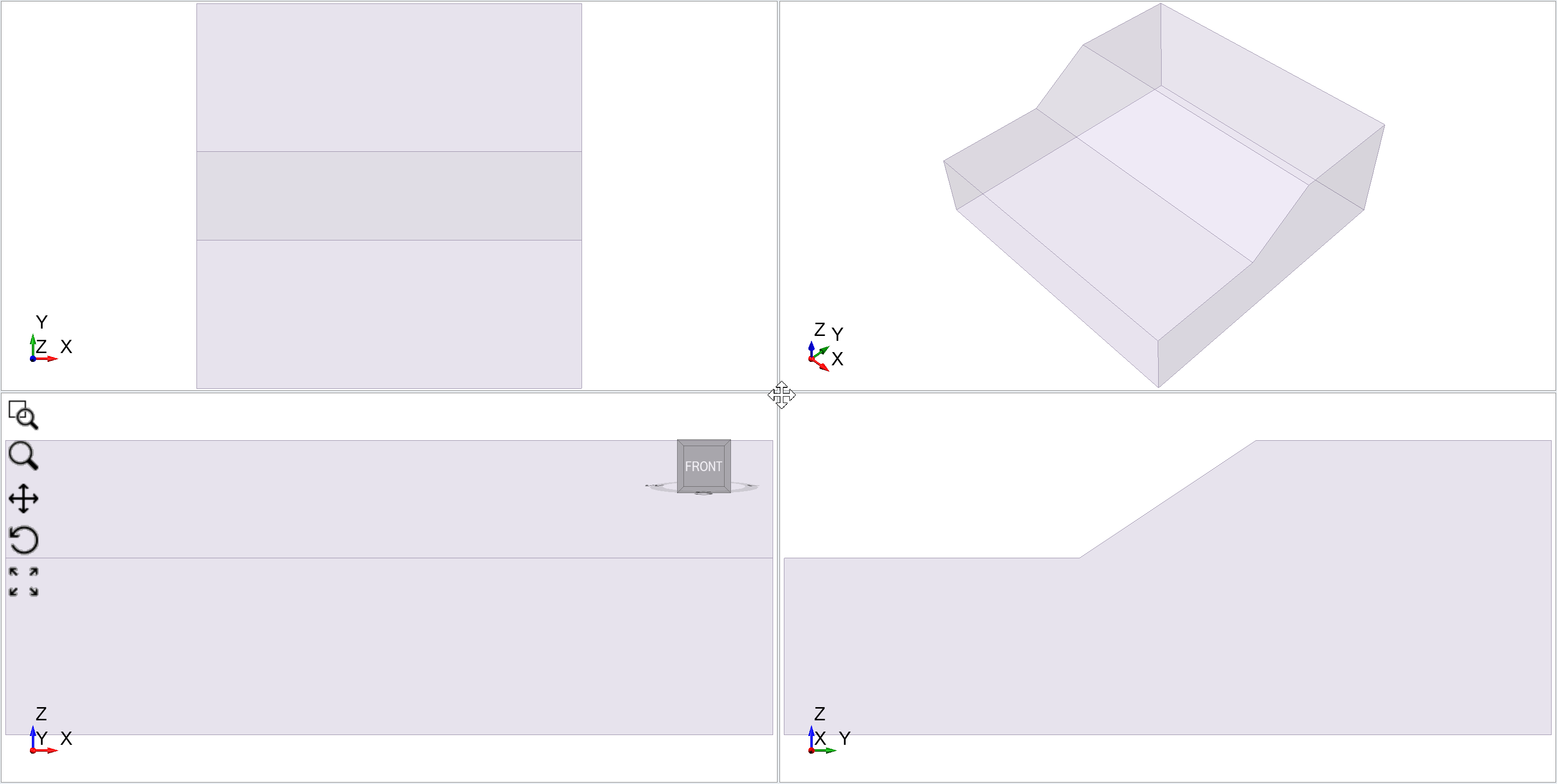
Yous have now added a two-dimensional profile of a gradient in the YZ plane. Printing F2 to view the zoomed images of the polyline.

In the sidebar Visibility pane, select the Polyline entity yous take just created.

Below the Visibility pane (in the Properties pane) change the Name to Slope Profile.

Extrude

With the Slope Profile notwithstanding selected we can extrude information technology to 3D.

Select: Geometry > Extrude/Sweep/Loft Tools > Extrude

You will run across the Extrude dialog.

Select the Close Book(south) checkbox at the top of the dialog. This ensures that the extruded volume volition be closed (i.eastward. non open-ended).

The Direction is based on the plane of the slope profile. Since we defined the coordinates in the YZ plane, the extrusion direction is the X direction.

Enter Depth = 130.

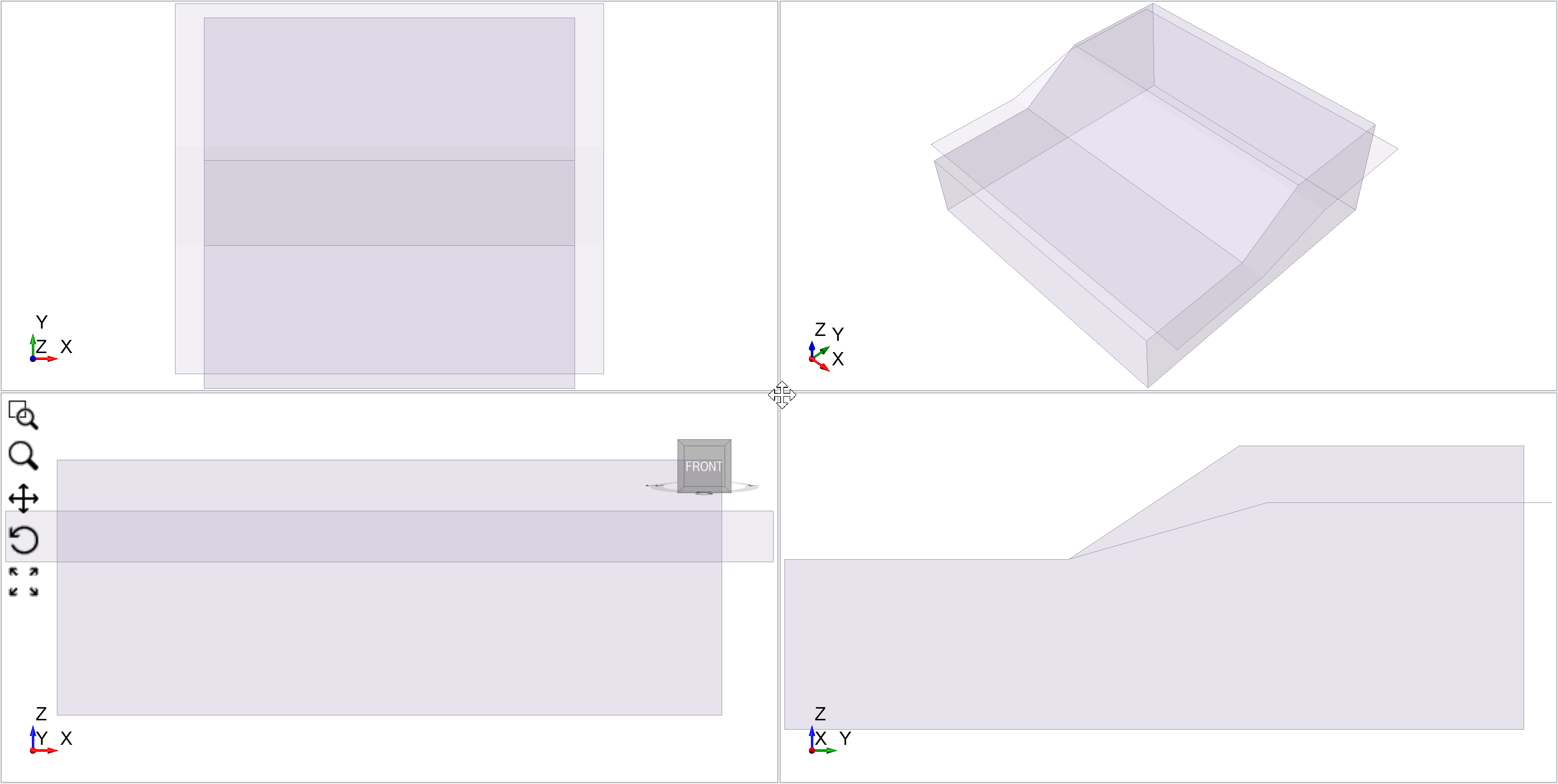
Selecting the Preview push will update the viewports with the new geometry. Check to run across if the extrusion parameters are correct. Select OK.

Your viewports should look as follows.

External Volume

Every Slide3 model must have an External book defined otherwise the extents of the slope geometry will be unknown.

In the Visibility pane select the Slope Profile_extruded entity we have merely created.

Select: Geometry > Set up as External.

The extruded gradient volume is now defined equally the External volume (also shown with a Lock icon).

In order to run Compute for whatever model you must define an External volume. Without an external volume the compute selection volition be disabled.

four. Define Materials

For the purposes of this tutorial our model will be composed of only one type of material (clay).

Select: Materials > Define Materials

Enter the following for Material 1:

• Proper noun = Clay,
• Unit of measurement Weight = 19,
• Cohesion = 5 kPa, and
• Phi = 30°

Select OK.

By default, Material ane is automatically assigned to all volumes within the External volume.

5. Skid Surfaces

Y'all tin can run an analysis without specifying slip surface information. Slide3 volition use default settings However let's take a look at the Skid Surface dialog.

Select: Surfaces > Slip Surface Options

The default slip surface options are:

• Surface Generation Method = Search Method
• Surface Blazon = Ellipsoid
• External Geometry Composite Surfaces = OFF
• Search Method = Cuckoo Search
• Surface Altering Optimization = ON

We will use the defaults for now. Select Cancel.

The Surface Type and Search Methods are very important features of the Slide3 analysis. These topics and all related topics can be found in Slide3'due south documentation page.

vi. Compute

Salvage the model before computing. And then, run the assay.

Select: Analysis > Compute

If the Compute option is disabled check that the External volume has been defined.

Compute should only have 2 or 3 minutes for this simple model.

When the Compute dialog closes y'all tin can view the Results.

7. Results

To view the results, select the Results Workflow tab .

The Global Minimum slip surface for the Bishop analysis will be displayed. The safety cistron (FOS) for the Bishop surface is well-nigh 1.15 as shown in the toolbar.

To view data contours on the slip surface select the Show Contours on the toolbar button . By default y'all will encounter Base of operations Normal Stress contours (i.east. the normal stress on the base of the columns).

To view the Janbu rubber factor select Janbu from the Method dropdown in the toolbar. The Janbu safety cistron is about 1.1.

To view other data contours, y'all can select dissimilar options from the Data dropdown carte du jour in the toolbar (eastward.g. Shear Stress).

Asymmetric Global Minimum for second Extruded Models

Yous may be wondering why the Global Minimum slip surface is not positioned at the center of the slope model, since the model is a 2D extrusion.

For a simple 2d extruded model, yous would look the results to be centered and symmetric. The reason that the results are not symmetric, is that the search methods (e.g. Cuckoo Search and Surface Altering Optimization) practice non know in advance that the model is symmetric, and therefore the terminal results can exist asymmetric as shown above.

For the purpose of obtaining symmetric results for second extruded models, the Symmetry selection in Project Settings can exist used. We will now demonstrate this option.

By default, the Symmetry selection is OFF. If the Symmetry selection is NOT used, then results for 2D extruded models can in full general exist non-symmetric (i.east. the Global Minimum slip surface may not be centered on the model, and the surface itself may exist asymmetric).

8. Symmetry Pick

To ensure symmetric results for second extruded models, you can use the Symmetry option in Project Settings. If the Symmetric Model checkbox is selected, the search results and global minimum sideslip surface will exist constrained to be symmetric along a user-defined vertical plane of symmetry.

• Select: Assay > Projection Settings and select the Symmetry tab
• Select the Symmetric Model checkbox
• Enter the post-obit XY values (65,0) for Point1, (65, 130) for Point 2 and select OK.
  

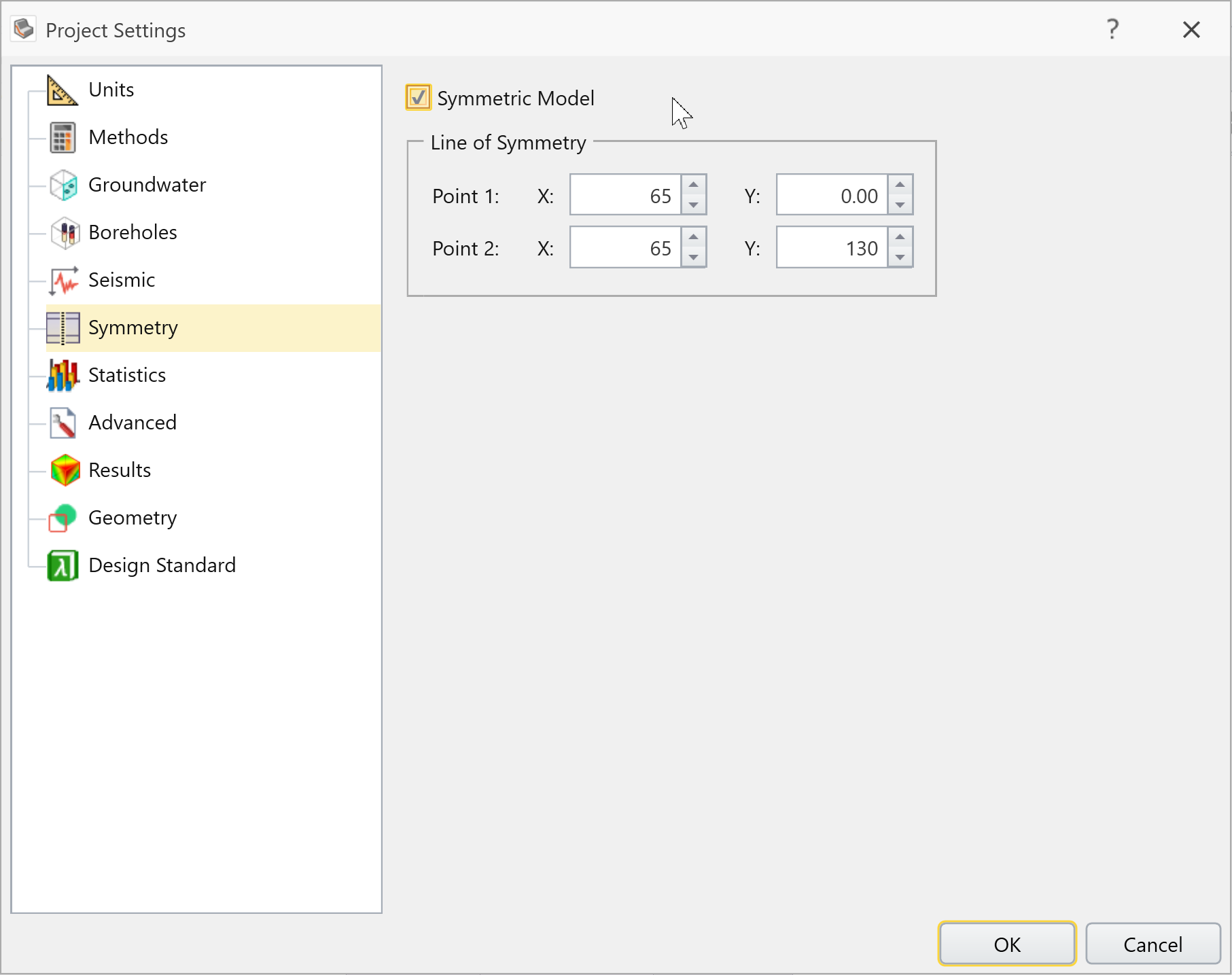
This defines a line of symmetry in the XY plane downwardly the center of the model.

Press F2 to Zoom All. If you select the Sideslip Surfaces tab, you will run into the line of symmetry displayed as a white dotted line above the model in the height and perspective views.

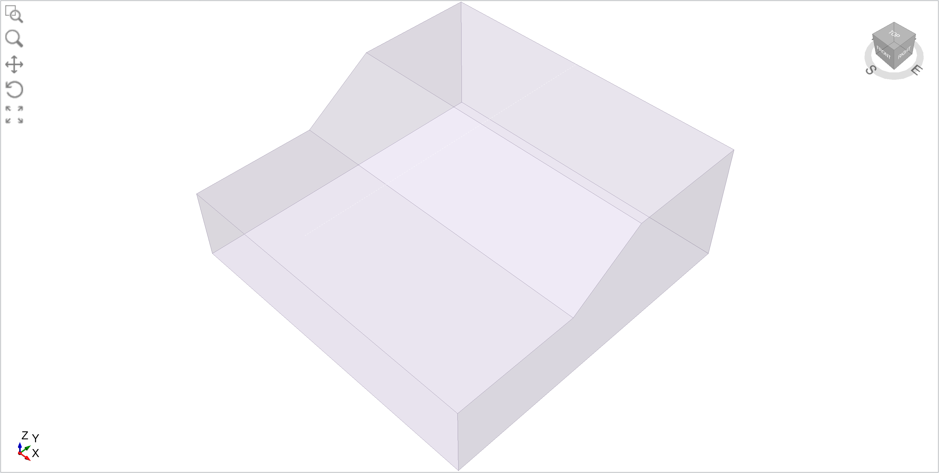
Line of symmetry displayed (white dotted line).

ix. Compute

Save the model earlier computing the analysis. Select: Assay > Compute to re-run the analysis with the symmetry option enabled.

10. Results

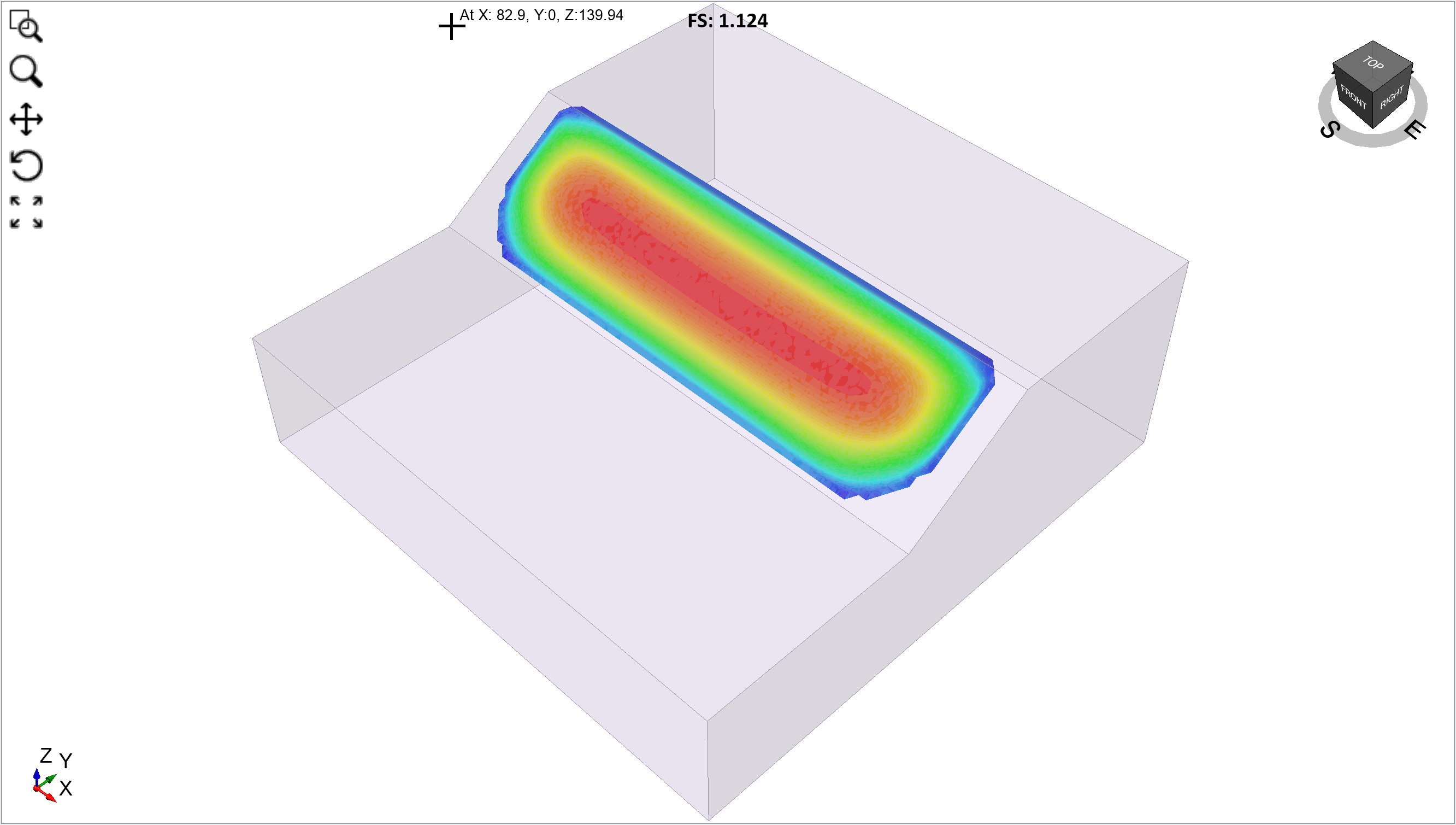
Select the Results workflow tab. Click on Show Contours icon in the toolbar .

Equally you can see the Global Minimum slip surface (with symmetry) appears quite different from the Global Minimum skid surface (without symmetry). The sideslip surface is longer, centered and symmetric, and the safety factor is slightly lower. The symmetric slip surface is essentially converging to a 2-dimensional solution (i.e. the skid surface tends to extend itself along the slope direction).

In full general, for symmetric 2nd extruded models, information technology is recommended that the Symmetry option should be enabled, using a line of symmetry down the middle of the model.

Safety Factor with Symmetry

When Symmetry is enabled, yous will commonly discover a different rubber factor compared to the non-symmetric results. All the same, the symmetric prophylactic gene might be higher or lower than the non-symmetric safety cistron.

You cannot generalize the event of symmetry on safety factor, specially with the Surface Altering search method. In some cases symmetry might give a higher prophylactic factor due to the greater restraint on the solution.

Show All Surfaces

This option reveals all of the slip surfaces that were calculated to reach the Global Minimum for both Bishop and Janbu. The slip surfaces are coloured co-ordinate to their safety gene.

Select: Interpret > Show All Surfaces

Select Filters in the Add together Filters section of the dialog. We are interested in viewing all the slip surfaces which had a FOS < i.2.

Enter the following:

• Information = FOS,
• Functioning = "<", and
  
• Max = ane.2
  

Select OK then Shut. We filtered out all simply the red skid surfaces (low FOS).

Bear witness Data on Plane (Safety Map)

Select: Translate > Prove Data on Plane > YZ

The Data on YZ Plane dialog is now open. you lot can change the X Location by using the cursor or by manually entering a value for X. Select OK.

To change the location of the safety map after you've created one, select Safety Map: YZ Airplane on Visibility pane, and under the Backdrop pane, click Edit Plane Options.

Y'all will see Data on YZ Airplane dialog once once more.

Cavalcade Viewer

Select: Translate > Cavalcade Data Viewer

This allows you lot to view detailed assay for whatever column of the Global Minimum surface.

11. Add Water Tabular array

Let's return to Geometry mode, add a water tabular array, and re-run the assay.

Select the Geometry workflow tab.

Select: Geometry > Polyline Tools > Describe Polyline

Select the YZ Plane Orientation

Select the Edit Table push in the Coordinate Input area of the sidebar.

Import by selecting and open the file 'Watertable_coordinates.txt' in the tutorial folder. Make sure to choose Tab under delimiter selection. Select OK.

Correct click and select Done.

In the Visibility pane, click on the Polyline entity and re-name it Water Table.

Select: Geometry > Extrude/Sweep/Loft Tools > Extrude

In the Extrude dialog, enter Get-go = -10 and Depth = 150. Practise Not select Close Volume(s), as the water table is just a surface. Select Preview to check the input parameters. Select OK.

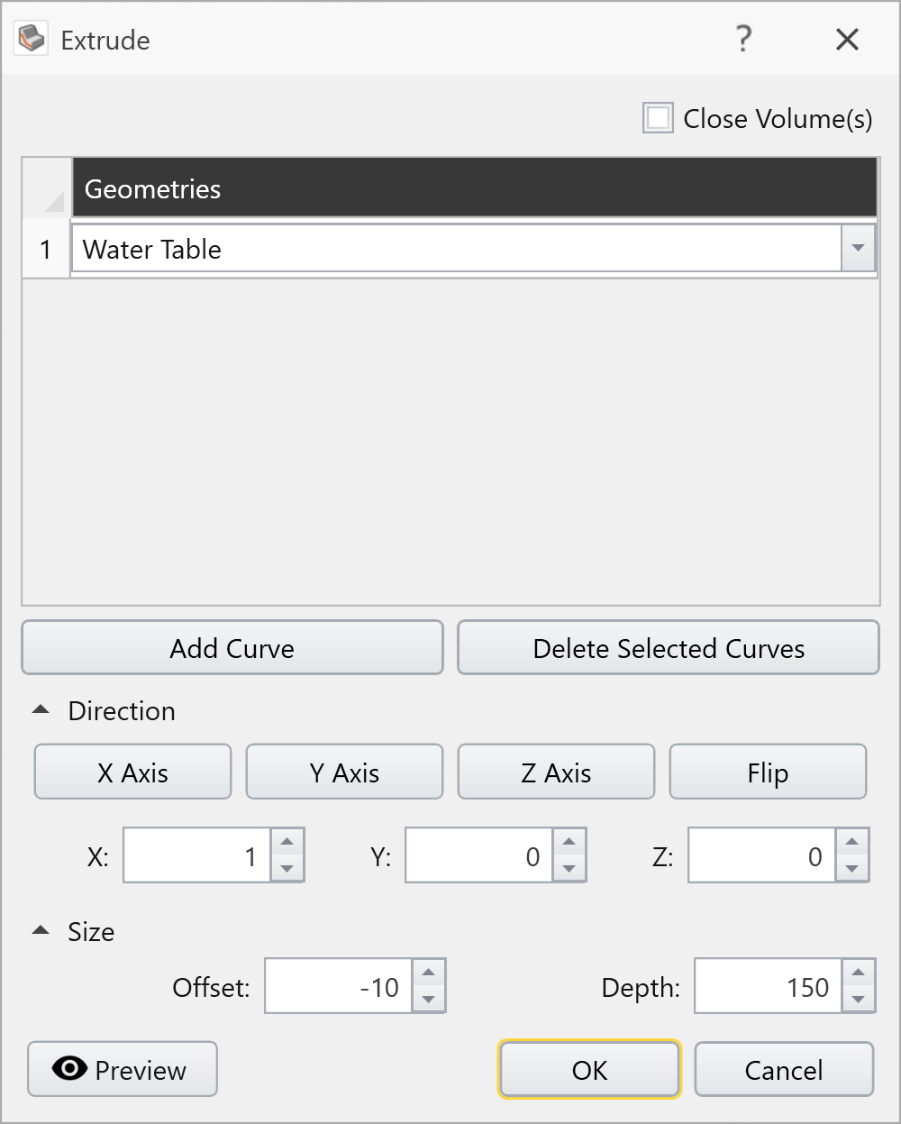
Annotation: the showtime and depth values of the extruded water table were used for brandish purposes, to brand the water table more visible on the model.

Add Water Surface

Although nosotros have added a polyline and extruded a surface, it is not actually a water table yet.

Select the Groundwater workflow tab.

Select: Groundwater > Add together Water Surface

Select OK to define the surface as a H2o Table.

You will then see the Hydraulic Assignments dialog. Select OK to assign the Water Tabular array to all materials:

The model should look as follows: To double check, slide along Transparency option in Properties pane to see the layers.

To check the h2o table consignment, get to the Define Materials dialog and select the Water Parameters tab for Material ane.

Equally you tin can see the Water Table is assigned to Material ane. Select Cancel.

Note: the default Groundwater Method can exist selected in Project Settings. This determines the initial setting for all materials. The Groundwater Method can also exist customized for each individual material in the Define Material Backdrop dialog.

12. Compute

Save the model.

Select: Analysis > Compute to re-run the analysis with the symmetry option enabled.

13. Results

Select the Results workflow tab

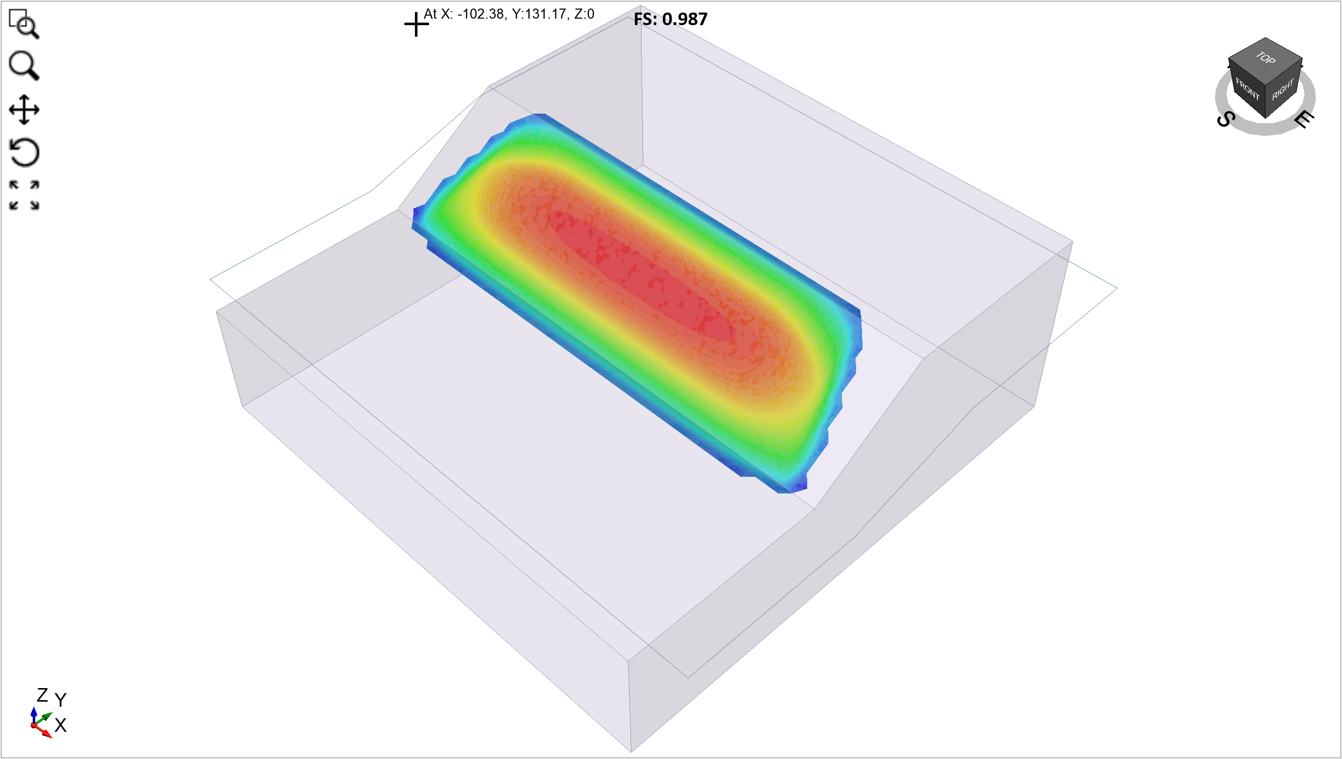
Select: Translate > Show Contours or select Show Contours icon in tool bar pane. You should run into the following.

The Bishop safety factor is now close to 1.0.

This concludes the tutorial.

roblesupose1987.blogspot.com

Source: https://www.rocscience.com/help/slide3/tutorials/2d-extruded-models/slope-with-water-table

Share this post